Introduction
Overview
Streams
Wrappers,Buffers
Console I/O
  Text Output 
     Demo 1
  Formatter/printf()
     Demo 2
  Tex 2t Input
     Demo 3
  Scanner
     Demo 4
File Class
  File I/O
  File Output-Text
     Demo 5
  Formatter to File
     Demo 6
  File Input - Text
    Demo 7
  Scanner - Files
     Demo 8
  File I/O - Binary
     Demo 9   Demo 10
File Chooser Dialog
  Demo 11
Character Codes
  Demo 12   Demo13
Object I/O
Types to Bytes
Stream Filters
Other I/O Topics
Exercises

Now that we have a simulator of the physics phenomena of interest (the dropping of a mass in a constant gravitational field), we want to add a a detector module to the program to simulate an experiment.

This kind of gravitational acceleration experiment is common in introductory physics courses. It is done by measuring changes in velocity of a dropped mass usually with a spark chart or photodiode setup. Here we simulate the latter type of experiment that measures when when the ball crosses fixed positions. Knowing the times and the positions along the path of the ball, we can calculate its change in velocity to obtain a measurement of g.

To insert our detector simulator into the code, we use a

• DropTestDetectApplet - new version of the applet/app class that assembles the program modules, including a detector.
• DropDetector - the detector object that simulates the measurement of the crossing times at points along the drop track.
• DropModelDetect - A new version of the physics model so that it now invokes a method in the detector class for each step of the ball.
• DropPanelDetect - A new version of the animation display that allows the detector to "draw itself".

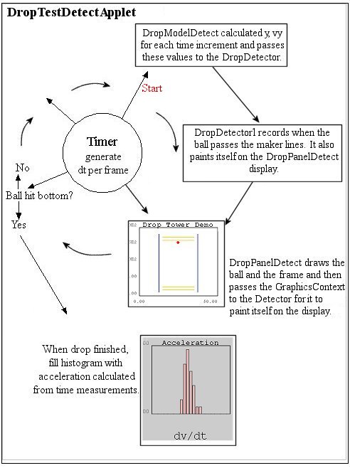
The simulator page shows the code. Figure 9.3 below shows the modifications to the process for the drop simulation combined with a detector:

Figure Phy.9.3: Similar sequence as in Figure Phy.9.2 but with the DropDetector class added. For each step in the simulation of the fall by DropModelDetect, the detector object is called and it notes the times when the ball touches the marker lines. The detector also paints itself on the animation frame. When the drop finishes, the applet gets the data for the time of the marker crosses, calculates the velocity for the two pairs of markers, and then uses the change in velocity to calculate the acceleration.

Detector Approximations

Note that for the detector we make one of those design decisions that affects the simulation's realism. For the sake of simplicity and program performance (i.e. to insure that it can complete the calculations within the animation frame time), we don't do a detailed simulation of the ball's shadowing of a beam of light on the sensor. We also don't simulate the signal from the sensor and its variations in crossing a threshold value to trigger the time setting. Instead, we just smear the time value according to a Gaussian distribution with a fixed standard deviation (e.g. SD=100ms.)

Furthermore, we just pick an arbitarary smearing. For a real experiment, you would look at the data from the detector to determine first if the measured values do in fact follow a Gaussian distribution and, if so, to adjust the simulation's SD to match what it produces.

Physics Approximations

You will also see that even for this simple physics simulation, there are some subtleties that arise. The program calculates increments in the dropped ball's position for increments in time. The detector measures when the ball crosses particular vertical coordinates. If we used a fixed increment dT for each step in the simulation (we will do this in the next section), then as the velocity increased the distance traveled within the DT period would increase. So our precision in marking when the ball passed the detector beams would grow increasingly worse as one examined longer drops. (The program just checks whether the position has reached or passed the detector lines for each increment.)

Here we try to fix this problem in two ways. Firstly, we divide the animation frame times into finer steps in time. (Note that more complex differential equations will almost always require finer integration stepsizes than the animation frame time for accurate results.) Secondly, we make the width of these fine time increments inversely proportional to the velocity, so that the precision in distance determinations remains roughly the same as the velocity increases.

              Tech
Histogram I/O
Hist I/O - Get/Set
  Demo 1
Hist I/O - Objects
  Demo 2
HistogramStream
  Demo 3
Filtering Data
  Demo 4
Exercises

           Physics
Physics Model
Simulation Design
Physics Simulator
  Demo 1
Experiment Design
Experiment Sim.
  Demo 2
Analysis
Expt. + Analysis
  Demo 3
Exercises