Java Tech - Chapter 11 : Physics

Below we show several examples of how our data simulation and analysis might be used. Though the drop example is very simple, the basic techniques here emulated what is done with modern complex experiments, which almost always require a simulation to obtain reliable results.

We set the mass to be dropped from 200cm and it crosses into the detector's sensitive region at 190cm. In the graphic shown below, the parameters are shown for the fit to the polynominal:

If an instrument offset is added to the position data, then the y₀ value will be displaced from 200cm.

Note that for the calibration run, the initial t=0 goes with the start of the detector sensitive region at 190cm. So the intercept fit to the calibration run data is at 190cm rather than 200cm.

Below we give 5 examples of different modes in running the simulator/analysis programs:

Demo 1: Drop with no Instrument Effects

DropGenCalSysErr

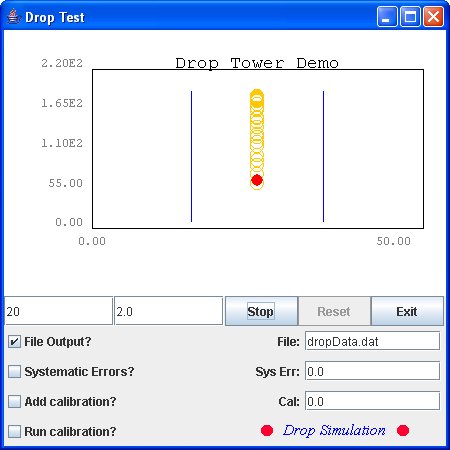
Normal run in which the data for 10 drops is written to a file named dropData.dat. The position values are smeared with a Gaussian using a sigma of 2.0, as input by the user in the second text field.

DropDataAnalysisCalSysErr

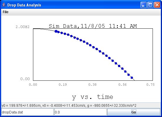
The user chose the dropData.data file with the file chooser dialog opened via the File drop down menu. Clicking on Go will cause the program to read in the data from the chosen file and fit the data points.

The blue points represent the average position for the 10 drops for each time increment. The std. dev. for the averages are barely visible as vertical red lines on each dot.

The dropped mass starts at 200cm and at zero velocity. It crosses into the detector sensitive region at 190cm. The fitted curve extends back to t=0 when the We see that the fitted parameters are consistent with these values. The g acceleration value determined by the fit is also consistent within the error with the 980 cm/s² value used in the simulation.

Demo 2: Run with Instrument Offsets

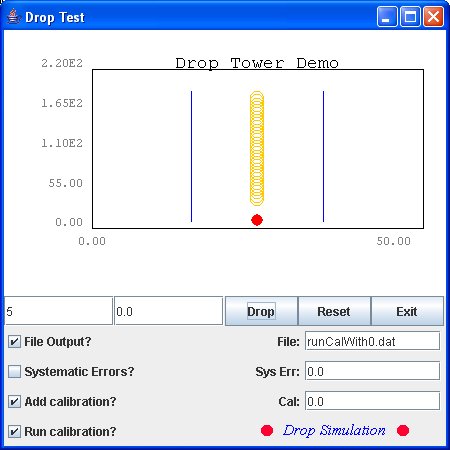
DropGenCalSysErr

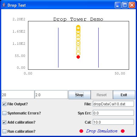
Add an instrument effect on the position data by choosing the "Add Calibration" checkbox and putting a value of 10.0 into the calibration constant value field. We send the data to a file named dropDataCal10.dat.

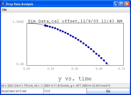
DropDataAnalysisCalSysErr

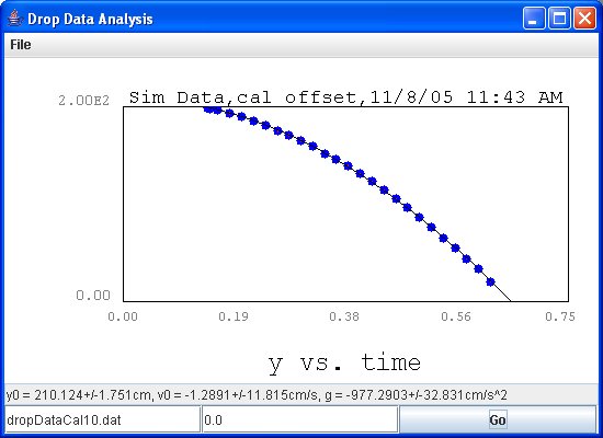
Because of the instrument offset, the fit intercept has been displaced by 10 cm upwards as compared to the fit in Demo 1.

DropDataAnalysisCalSysErr

We can rerun the analysis but use a calibration constant of 10.0 to subtract from the data. Now the fit intercept is back at the correct 200cm position.

Demo 3: Calibration Run with no Instrument Effect

DropGenCalSysErr

Do a calibration run with 0.0 value put into the calibration constant field. Send the data to a file named runCalWith0.dat.

DropDataAnalysisCalSysErr

A fit to the calibration run data shows a straight line and an intercept at 190cm, which is the position where the detector sensitive region starts.

Demo 4: Calibration Run with Instrument Effect

DropGenCalSysErr

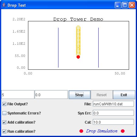
Do a calibration run with 10.0 value put into the calibration constant field. Send the data to a file named runCalWith10.dat.

DropDataAnalysisCalSysErr

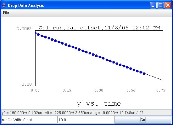
A fit to the runCalWith10.dat calibration run data with a calibration of 10 subtracted from the data shows a straight line and an intercept at 190cm.

Demo 5: Run with Systematic Error

DropGenCalSysErr

Here we generate drop data with the systematic error checkbox selected and a value of 1.2 put into the systematic error field. This will cause the time step between position measurements to be expanded by 20 percent. The data goes to a file named runSysErr1_2.dat.

DropDataAnalysisCalSysErr

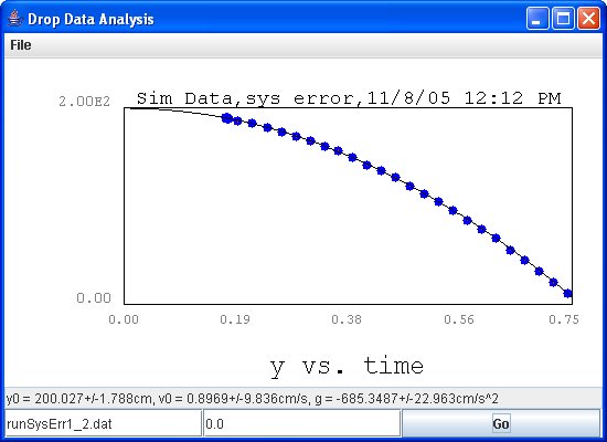
A fit to the runSysErr1_2.dat shows that the intercept and initial velocity values are still as expected but now the acceleration has gotten significantly smaller. This is due to the fact that the mass took longer to reach each measurement point.

In a more complex experiment, many such variaions in different aspects of the experimental system, even those that are expected to be well understood and fixed, should be studied to see if they affect the results signficantly.