| Home : Map : Chapter 1 : Java : Tech : Physics : |
|
Physics Simulation and Analysis
|
| JavaTech |
| Course Map |
| Chapter 1 |
| Introduction History What is Java? Versions Java 5.0 Features Java Process Tools Documentation Compatibility Getting Started Simple Applet Simple Application Starters Exercises |
|
Supplements |
| About
JavaTech Codes List Exercises Feedback References Resources Tips Topic Index Course Guide What's New |
Simulations of physics phenomena provide useful demonstrations that help to develop intuitive understanding. However, simulations are not just for the classroom but are essential tools for carrying out modern experiments.
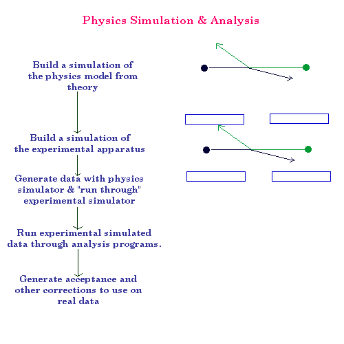
To design an experiment, run it, and understand the results, a simulation is not an accessory but a necessity. The phenomena under investigation in modern physics are too subtle and the experiments too complicated to attack with only analytical tools. This diagram shows, for example, the essential steps in the simulation and analysis of a particle collision experiment:

Here two particles collide and scatter. A set of detectors is placed to detect the particles after they scatter. Perhaps thousands or even millions of such collisions will take place in the course of the experiment.
The detectors only cover part of the area into which the particles scatter. So to determine the important aspects of the interaction, such as the scattering cross-section, corrections will have to be made for the limited coverage of the total solid angle and the inefficiencies in the detector sensitivity.
Note: In an experiment simulation, we must simulate not only the physics phenomena of interest, such as the collision of the two particles, but also the interaction with the experimental apparatus. In this case, the simulation must also take into account the interactions of scattered particles with the detector materials.
Using this simulation, we determine the acceptance correction: the percentage of the collisions that were accepted or sensed by the detector. This can involve geometric limitations of the detector, such as what portion of the solid angle that it covers and what dead spots it has.
In our simulation we control how many collisions take place, so we can simply compare the generated number of events to the ones detected. Then for the real experiment we apply these acceptance correction factors to the data from the detector to obtain the scattering parameters of interest.
Of course, one must be sure that the simulation is as close to the true system as possible. Otherwise, the corrections to the measured values will be incorrect! A check on the simulation is to first measure the values of parameters that are precisely known and see if the measurements agree with the known values.
For example, here the collisions could first be carried out at lower energies where previous experiments measured the scattering cross-sections with other detectors at other accelerators. If the lower energy measurements agree with the values obtained in these previous experiments, then one can feel more confident about the corrections to the data at the higher energies.
It is not uncommon in large high energy physics to create two simulation packages. One program will carry out a highly detailed simulation of every detector subsystem at a very fine scale. A careful comparison of the simulation to the actual hardware performance will provide confidence that the hardware is well understood.
However, such fine grade simulations will typically run very slowly. For analysis of real data one often needs to compare the results to simulated distributions with high statistics to see the signal above the background. So one approach is to create a second simulation that uses much coarser approximations to the detectors but runs much faster. For example, after a track traverses a wire chamber, rather than following the ionization as it drifts to the sense wire and simulating the rest of the detection process, the coarse simulator will simply assign an average error bar to the position coordinate at the location of that wire. The coarse simulator would be "tuned" to the detailed simulator (as well as to calibration measurements made on the real detectors, perhaps with a test beam) to provide the same general level of accuracy for the various detector measurements such as track finding, momentum determination, energy determination of neutral charged particles, and so forth.
Latest update: Dec.10.2003
|
Tech |
|
Physics |